Introduction to Data Science

With a number of companies growing every year, the world has entered into the genre of big data. That is the reason why the storage for the same also increased. It has become a major challenge as well as concern for these industries to save those data perfectly without any issue.  The major issue was to build the framework of data and bring out more solutions to store the same. As Hadoop with other frameworks has come into being, solving the storage problem has become easier. Now the main focus lies on the processing of the same data. Here comes the story of Data Science! You go to watch movies right? Well, all the graphics and the overdo turn into reality through the Data Science process. The future of AI or Artificial Intelligence as you all know lies with Data Science. Thus, it is necessary to understand the meaning of Data Science and how it is creating a niche for the business.

Questions that arise in our minds

Well, will the Data Science coming more and more into the market and dominating it, there are some questions that linger into the kinds of people. Here are some;

• Why Data Science is needed most?
• What is the meaning of Data Science?
• What is the difference between Data Science and Data Analysis?
• The lifecycle of Data Science.

All these questions have answers that will be discussed vividly below. This will help to gain in-depth knowledge of the field.

Why Data Science is needed most?

Well, earlier whatever data that we used was a structured one and very miniature in size. These could be easily analyzed through simple tools like BI. But with the development of technology, these days, data is mostly unstructured which was structured earlier. As per research, by the year 2020, more data will become unstructured and uncontrollable. These need to be checked immediately.

Now you will question as in from where all these data is generated? Well, all these data is gained from an immense number of sources such as- text files, forms in multimedia, sensors, financial logs, various instruments and so on. It is beyond the work of simple BI tools to process this large quantity of data in such varieties. This is the reason more complex as well as advanced and modern tools of analysis are required for understanding and bringing correct as well as meaningful results out of the same. This has made Data Science so much popular amongst the people and the companies.

With Data Science, it has become easier for the companies to bring out instant information of customers such as- the earlier browsing history, his purchase history, his carts collections, his age and the income group he falls into. All these data were there earlier too but it was not so easy to generate the same. With the advancement of Data Science, data gained is vast and in variety. One can have effective training of the models and also recommend the product to the consumers in short. These automatically arouse the purchase rate which further increases the business of that particular firm.

Role of Data Science in Decision Making

The role of Data Science in making larger decisions for the company is very important. These days, you get to have self-driving intelligence-based cars that could actually collect all the live data from the in-built sensors. There are lasers, radars, and cameras that automatically create an invisible map of the surroundings and based on the same, the automobile can decide when it will speed up when to lower the speed if to overtake or not, where the turning point is. All these are done via an advanced system of machine learning algorithms.

Not only this, you can use this wonderful technology in predictive analysis too. For forecasting of weather, you need Data Science too. Data Science is required to collect data from ships and aircraft, from radars and satellites and used for building various models too. This information helps in the forecasting of weather and can also predict if there is any coming of natural calamity. Thus, appropriate measures can be taken from beforehand too which will cause the saving of a lot of lives.

Domains where Data Science is creating a lasting impression

Data Science is now mostly used in major fields. Here is the detail;

• Marketing channels use data science to cross-sell, up-sell and predict lifetime valuation of various customers.
• Travel uses Data Science majorly so as to predict flight delays, major dynamic pricings, customers traveling, etc.
• The Healthcare genre uses Data Science to understand the prediction of disease and whether the medications will be effective.
• The social media field uses Data Science to understand digital marketing and analyze the sentiments of various people.
• The Sales genre also uses Data Science effectively to maintain discount offerings and maintain the demand forecasting process.
• The Automation field also uses Data Science to make self-driving mechanisms such as cars and other machinery.
• Credit and Insurance genre uses Data Science to detect fraud and risk and claims prediction too.

Now that we know all about Data Science, it is necessary to know what Data Science exactly means.

What is Data Science?

Data science can be explained as the science that deals with the identification, representation, and extraction of needful and meaningful information from a pool of data that are useful for the further growth of the business. It is actually a mixture of programming and analytics that works on unstructured raw data to create finely chopped useful pieces. The presence of a large amount of data with various structure and purpose, it is quite difficult to choose the most appropriate one. It is in this phase that the data engineers set up databases and data storage to ease data mining.

In a business firm, the amount of data creation increases rapidly and the data scientist helps such organizations to convert the raw data into valuable business data. Data extraction converts the unstructured data into pure and polish data that will be useful for further processing. The important characteristics that a data engineer should possess are good knowledge of machine learning, statistical skills, analytics, coding, and algorithmic experience.

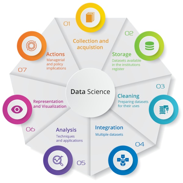
Taking up a data science career means you have to make yourself expertise in deploying statistics and deducting reasoning. The best way to get the best result is going through several steps that every data scientist should obey. It includes:

• Understanding the problem
• Collecting enough data
• Processing the raw data
• Exploring the data
• Analyzing the data
• Communicating the results

A mixture of various tools and algorithms, machine learning features and principles, the target of data science is to find out the patterns underneath from unstructured data. A data analyst builds business administration and analyses it with detail explanations whereas a data scientist deals with machine learning issues and modern algorithms. Through a data analyst, one can understand the total processing mechanism of data but a scientist is not only involved in exploratory details but also uses major modern algorithms to understand the need for a certain program in the near future. A good Data Scientist is always looking at certain data via many angles. Thus, Data Science is majorly used to make important decisions as well as analyses through predictive analytics or prescriptive analytics and also machine learning.

Predictive Analytics

If there is a model through which one can understand the nature of a certain event of the future, predictive analytics is used. If a certain company is providing its customer money on a credit basis, the probability of consumers making use of future payments of credits at a certain time should be a matter of concern for that company. Through this, one can easily build a model that will act on predictive analytics on the basis of the payment history of that particular consumer so as to predict if the on-time payments will be made perfect in the future or not.

Prescriptive Analytics

For prescriptive analytics, you need models that have the strength of taking a major decision on its own and also have the ability to change and modify with major parameters. It is all about providing the correct advice and a range of certain actions with the best outcomes. A good example is always better to make the scenario easier. Say, for example, Google’s self-driving car. All data collected by these vehicles are used to train the self-driving automobiles for which one can also run major algorithms over it so as to add intelligence to it. This helps the car to take major decisions as in when to change gear, when to turn, when to slow and speed, etc.

Machine learning mechanism

For example there is a huge number of transactional data of any financial company. You need to build up a good model so as to understand the next trend of the same, then use machine learning algorithms. This is known as supervised learning procedure as one has the complete data through which one can easily train the machines.

Pattern Discovery through Machine learning

If there are no segments on which one can make solid predictions, one can easily find hidden segments in the data with meaningful predictions. With no defined labels, this is termed as the unsupervised model. Thus, the common system of the algorithm used here is clustering. For example- A telephone company wanting to establish a perfect network through proper towers in an area will use this method of clustering to find exact tower locations. This will help all users to get perfect signal strength. So how do Data Science and Data Analysis differ?

Well, Data Analysis has the descriptive detail as well as a prediction at a certain label. But Data Science is more about Machine learning and Predictive casual analytics system.

The lifecycle of Data Science

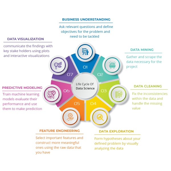
It is necessary to understand the perfect lifecycle of data science without running into any conclusion and data collection procedure. This will help in the smooth running of any project.

PHASE 1 – DISCOVERY:

For the smooth running of the project, it is necessary to understand the different specifications, the major needs, priorities, and the exact budget. In this process, one predicts and analyses the required assets in terms of time, data support system, people, and technology to be used and many other which is important. Framing the problem of the business is another major thing to be done here.

PHASE 2 – PREPARATION OF DATA:

To perform certain analytics for the total duration of a project, an analytical sandbox is required in this phase. Through this one can easily explore, process and prepare proper data before the modeling. Also, Extraction, Transformation, loading is performed through this phase. For proper transformation, visualization and cleaning of data, R is used here which will further help in spotting the outliers and making a good relationship through various variables. As the data is completely cleaned and prepared, the time comes to perform analytics on it.

PHASE 3 – PLANNING OF MODEL:

Various techniques, as well as methods, are determined here which will help in detecting major relationships through variables. All these relationships will make a base for most algorithms that are to be implemented in the next phase. Through this, one will apply Exploratory Data Analytics through the usage of normal formulas in statistics and various visual tools.

Here are the major planning tools;

• R is a major tool that has a new set of modeling requirements and helps to make a good environment for preparing models on interprets.
• Analyzing services of SQL is another important tool that is used to access various data from system Hadoop and is used to create continuous model flow designs.

PHASE 4 – MODEL BUILDING:

This phase is used to maintain certain sets of data for various training as well as testing needs. Here, it is perfectly understood whether the tools that already exist are enough so as to run various models or if there is a need for major robust surroundings such as fast processing forms. Lots of learning techniques are analyzed here such as- association, classification as well as clustering to build a perfect model. Model building is achieved through;

• WEKA method
• SASA Miner
• SPCS Model
• Matlab process
• Alpine Miner system
• Statistica system

PHASE 5 – OPERATIONALIZE:

This phase helps in delivering major reports, important briefings and coding, and other technical documentation. Thereafter, a pilot project is made through an actual production environment. This helps in providing clarity of performance and major constraints over a minimum scale before any deployment.

PHASE 6 – COMMUNICATE RESULTS:

It is very much necessary to understand if one has been able to make to the goal that one had planned earlier in phase one. Thus, the last phase is used to identify all major key results and communicate each to all the stakeholders and give out the results of the said project. It might be a successful one or a failure one depending on the features developed in the first phase.

All said and done, Data Science has become one of the most important tools nowadays and it won’t be predicted wrong if one says that future technology belongs to Data Science. By the end of the year 2020 or so, Data Scientists will be most needed and with more and more companies growing with huge data, there will be opportunities that will help in making major business decisions. With Data Science being the most important technology, the world is soon going to take a major revolution in the field of Technology when huge data kept in safety will not be a problem anymore. Thus, it is required for a Data Scientist to be highly skilled and to be motivated so that he could solve the problems at ease.

Subsets of Data Science

The different subset of data science includes:

Data Analyst: It includes the analysis of data using various tools and technologies. It can be done using various programming languages.

Data Architect: He performs the high-level strategies that include integrating, centralizing, streamlining and protecting the data. He should have high authority over various plans and should have good knowledge of various tools like Hive, Pig, and Spark, etc.

Data Engineer: He is supposed to work with a large amount of data where the logical statistics and programming languages club each other. The data engineer should have a software background.

Data Science – the three Skillset

Data science can be called a club of three major skills which include mathematical expertise, hacking skills (technologies) and strong business acumen.

Mathematical Expertise

Before approaching the data, the data scientist should create a quantitative strategy through which exact dimensions and correlations of data can be expressed mathematically. The solutions to many business problems can be solved by building analytical models. It is a misconception that the lion’s share mathematics includes the statistics. But, the fusion of both classical and Bayesian statistic is will be helpful.

Hacking Skills (technologies)

Here we don’t mean breaking a computer and taking out the confidential data. The hacking here refers to the clever technical skills that will make the solutions as faster as possible. Many technologies are very important in this area. Many complex algorithms are related to each task and hence the deep knowledge in core programming languages is a must. Data flow control is another sophisticated area. The man dealing with the problem should be tricky enough to find the loops and high dimensional cohesive solutions.

Business Acumen

A data scientist should have a solid awareness of tactical business traps. He will be the one person in the organization that works closely with the data and hence he can create great strategies that will solve very minute problems.

Top tools of Data Science

It is categorized as:

• R Programming
• SQL
• Python
• Hadoop
• SAS
• Tableau

Difference between Data Science and Business Intelligence

Data Science is often confused with Business Intelligence but if understood well, one would know that there is a perfect difference between the two.

Business Intelligence predicts as well as analyses the earlier data so as to find the proper insight which will describe business trends. Through BI, one can easily collect data from internal as well as external sources and prepare it well to run major queries on it. This will help in creating dashboards which will help in answering the problems.

But Data Science is a more advanced concept. With its exploratory process, it has the power to understand past data or the current data and make the future results with the target of correct decisions. The “what” and “how” questions are answered here perfectly.

BI is much-unstructured data such as- SQL or Data Warehouse. But Data science is structured and unstructured such as- Cloud data, SQL, NoSQL, etc. the approach of BI is through statistics and visualization and the approach of data science is through machine learning and linguistic programming. BI focuses more on the past and present but Data Science focuses on Present and future. BI uses tools such as Pentaho, Microsoft BI, R, and QlikView. Data science uses RapidMiner, BigML, Weka, and R too.

Differentiating Data science from Big data

Big data consists of structured, unstructured and semi-structured data whereas data science deals with programming, statistical and problem-solving techniques. In big data, we will be using various methods to extract meaningful insights from large data. In data science, we will be using the above-mentioned techniques to solve the problems. Irregular and unauthorized data will be dealing with data science.

The importance of data science is increasing day by day. There are many factors that enable growth. The evolution of digital marketing is an important reason. The data science algorithms are used in every strategy in digital marketing to increase the CTR. Also, data science will increase performance. It will give way to real-time experimentation. One who can please the customers will win the business. Data science will create the best way for the same.

Sample Data Science Use Case

Till now we have introduced you to the various aspects of data science from a theoretical point of view. Now let’s take a simple data set and try to explore the underlying pattern of the data. Here we will refer a data set of patients who had undergone surgery for breast cancer. These data set has been collected between 1958 to 1970 at the University of Chicago’s Billings Hospital.

We will use python for this use case. As discussed above for any typical data science use case the starting point is a collection of the data, the data is then going through phases called data cleaning, data preprocessing, exploratory data analysis, model development, production deployment, offline and online testing, etc. based on the complexity and domain of the use case. For the sake of simplicity, we will use this “haberman Dataset”, which you can say a “Hello World” of the data science world.

Import Necessary Libraries

Libraries are basically the python packages. The reason python is so popular among the data science community is the availability of a vast repository of scalable and open-sourced packages. Now let’s import the necessary packages first

#importing necessary Libraries           
# pandas is a python library which provides data structure to 
read, write and manipulate structured data
# Seaborn,matplotlib are python libraries used for data visualization
and Exploratory data analysis
import pandas as pd
import seaborn as sns
import matplotlib.pyplot as plt
from sklearn.preprocessing import Normalizer
from sklearn.linear_model import LogisticRegression
from sklearn.model_selection import train_test_split
from sklearn.metrics import precision_score,recall_score,accuracy_score
#Loading Haberman Dataset
hman=pd.read_csv('Haberman.csv')

Preliminary Analysis of the Data

Now when we are done with loading the data in the memory, we will seek answers for the following questions in the data. Let’s first form the preliminary level of question sets we want to explore

1. How do the data look?
2. What is the shape of the data? How many data points we have?
3. What type of problem statement we can make from the data?
4. What are the independent and dependent variables?
5. Is the data set balanced?
6. Can we infer anything useful from the data using high-level statistics?
   Now we will go through each of this one by one to get an answer.

How do the data look?

In [10]:
# Overview of the data - top 5 rows
hman.head()

Out[10]:

s.no	Age	year	positive_axillary_nodes	survival_status
0	30	64	1	1
1	30	62	3	1
2	30	65	0	1
3	31	59	2	1
4	31	65	4	1

What is the shape of the data? How many data points we have?

In [9]:
# shape of the data in the format of(number of data points, number of variables)
hman.shape
Out[9]:
(306, 4)

The data set have 306 data points with 4 variables, which are the columns of the data set. Following are the variables of the data set.

In [11]:
hman.columns
Out[11]:
Index(['Age', 'year', 'positive_axillary_nodes', 'survival_status'], dtype='object')

“Age” refers to the age of the patient at the time of the operation, “Year” is the year of operation, “Positive axillary nodes” refers to the number of positive axillary nodes in the breast. It is an important parameter to identify the spread of breast cancers. “Survival status” refers to the survival status of the patient after five years of undergoing surgery and treatments.

What type of problem statement we can make from the data?

We can form our objective to predict a patient who has undergone surgery for breast cancer will survive 5 years or not based on the patient’s age, year of operation and number of axillary lymph nodes. In the literature of data science this is called a classification problem. Here we have two classes: class 1(Survived), Class 2(Not survived). Let’s make the class labels meaningful (Yes, No) for the sake of understanding.

# modify the target column values to be meaningful and categorical
hman['survival_status'] = hman['survival_status'].map({1:"yes", 2:"no"})
hman['survival_status'] = hman['survival_status'].astype('category')
# printing top of modified data
print(hman.head(2))

Output

	Age	year	positive_axillary_nodes	survival_status
0 30 64 1 yes	3	64	1	yes
1 30 62 3 yes	3	62	3	yes

What are the independent and dependent variables?

The independent variable is the variable whose value we want to predict, like in our case ‘survival status’ will be our independent variable and the rest of the variables will be our dependent variables. Based on our dependent variables (X) we want to predict the value of the independent variable (Y). It is a binary classification (as we have two classes) problem.

Is the Data set imbalanced?

A data set is called a balanced data set if a number of data points belong to each class is the same. In many real-world problems that have high dimensional data, the imbalance is a serious problem and needs to be addressed properly.

# Number of Datapoints wrt 'Survival_status'
hman['survival_status'].value_counts()

Out[16]:

yes    225
no      81
Name: survival_status, dtype: int64

The data set contains 225 data points belong to class ‘Not Survived’ and 81 data points belong to ‘Survived’. So Haberman data set is an imbalanced dataset.

Can we infer anything useful from the data using high-level statistics?

Pandas provide a function called ‘describe’ which can be used to get the high-level statistics (Mean, Standard deviation, Quantiles of the numerical variables) of the data set

# High-Level Statistics
print(hman.describe())

Output

	age	year	positive_axillary_nodes	survival_status
count	306	306	306	306
mean	52.457516	62.852941	4.026144	1.264706
std	10.803452	3.249405	7.189654	0.441899
min	30	58	0	1
0.25	44	60	0	1
0.5	52	63	1	1
0.75	60.75	65.75	4	2
max	83	69	52	2

In the above statistics we can observe the following points:

1. The age of Patients varies from 30 to 83 with a mean of 52.
2. 25% of Patients have no axial nodes, 50 % of patients have one axial node, 75 % have four axillary lymph nodes.
3. 75% of patients diagnosed with breast cancer are above 60 years old.

Please note we can not come to any conclusions based on these points, these are just preliminary observation about the data and needs to go through more concrete statistical tests (like hypothesis testing) to infer any statistical significance.

Univariate Analysis

‘Uni’ means one. Univariate analysis is used to graphically test the characteristics of a single variable. Let’s perform a quick univariate analysis of our independent variable ‘survival_status’.

Using Histograms

In [10]:
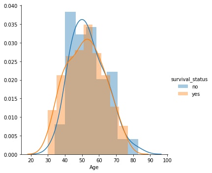
# plotting probability distribution of survival status w.r.t Patient's Age
plt.close()
sns.FacetGrid(hman,hue='survival_status',size=5).map(sns.distplot,'Age').add_legend()
plt.show()

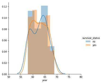
# plotting probability distribution of survival status w.r.t Patient's Year of Operation
plt.close()
sns.FacetGrid(hman,hue='survival_status',size=5).map(sns.distplot,'year').add_legend()
plt.xticks([50,55,60,65,70,75,80])
plt.show()

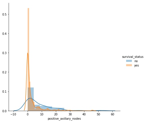
# plotting probability distribution of survival status w.r.t Patient's 
number of positive axillary lymph nodes
plt.close()
sns.FacetGrid(hman,hue='survival_status',size=6).map(sns.distplot,'positive_axillary_nodes')
.add_legend()
plt.show()

Observations

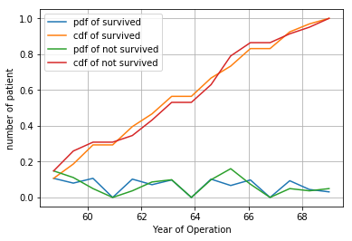
1. We can not easily separate survival status based on age or year of operation.
2. We can separate survival status comparatively better wrt. axillary lymph nodes.
3. Patients with 0 to 2 axillary lymph nodes have the highest probability of survival after 5 years.

Using Probability Distribution Function

In [19]:
# CDF of the survival status w.r.t Patient's Age
label = ["pdf of survived", "cdf of survived", "pdf of not survived", "cdf of not survived"]
hman_survived=hman.loc[hman['survival_status']=='yes']
hman_not_survived=hman.loc[hman['survival_status']=='no']
counts,bin_edges = np.histogram(hman_survived['Age'],bins=15)
pdf=counts/sum(counts)
cdf=np.cumsum(pdf)
plt.figure(1)
#plt.subplot(211)
plt.plot(bin_edges[1:],pdf,bin_edges[1:],cdf)
#plt.subplot(212)
counts,bin_edges = np.histogram(hman_not_survived['Age'],bins=15)
pdf=counts/sum(counts)
cdf=np.cumsum(pdf)
plt.grid()
plt.plot(bin_edges[1:],pdf,bin_edges[1:],cdf)
plt.xlabel('Age')
plt.ylabel('number of patients)
plt.legend(label)

Out[19]:

<matplotlib.legend.Legend at 0x237198437f0>

# CDF of the survival status w.r.t Year of Operation
counts,bin_edges = np.histogram(hman_survived['year'],bins=15)
pdf=counts/sum(counts)
cdf=np.cumsum(pdf)
plt.plot(bin_edges[1:],pdf,bin_edges[1:],cdf)
counts,bin_edges = np.histogram(hman_not_survived['year'],bins=15)
pdf=counts/sum(counts)
cdf=np.cumsum(pdf)
plt.grid()
plt.plot(bin_edges[1:],pdf,bin_edges[1:],cdf)
plt.xlabel('Year of Operation')
plt.ylabel('number of patient')
plt.legend(label)

Out[21]:

<matplotlib.legend.Legend at 0x23719c6b9b0>

#CDF of the survival status w.r.t axillary lymph nodes
counts,bin_edges = np.histogram(hman_survived['positive_axillary_nodes'],bins=15)
pdf=counts/sum(counts)
cdf=np.cumsum(pdf)
plt.figure(1)
#plt.subplot(221)
plt.plot(bin_edges[1:],pdf,bin_edges[1:],cdf)
#plt.subplot(222)
counts,bin_edges = np.histogram(hman_not_survived['positive_axillary_nodes'],bins=15)
pdf=counts/sum(counts)
cdf=np.cumsum(pdf)
plt.grid()
plt.plot(bin_edges[1:],pdf,bin_edges[1:],cdf)
plt.xlabel('axillary_lymph_nodes')
plt.ylabel('number of patient')
plt.legend(label)

Out[25]:

<matplotlib.legend.Legend at 0x2371ace47b8>

Observation(s)

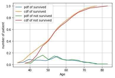
1. 80% of survived patients are aged less than equal to 64.
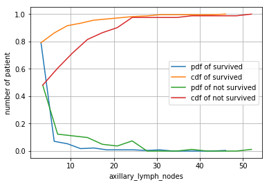
2. Patients with more than 47 axial lymph nodes have not survived.
3. Patients operated with the age of more than 77 years have not survived.
4. 80% of survived patients have less than 4 axillary lymph nodes.

Using Boxplots

In [27]:
# Boxplot of the survival status w.r.t patient's age
sns.boxplot(y='Age',x='survival_status',data=hman)
plt.show()

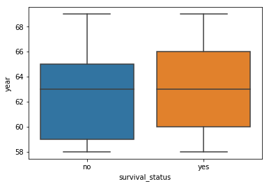
# Boxplot of the survival status w.r.t year of operation
sns.boxplot(y='year',x='survival_status',data=hman)
plt.show()

# Boxplot of the survival status w.r.t number of positive axillary lymph nodes
sns.boxplot(y='positive_axillary_nodes',x='survival_status',data=hman)
plt.show()

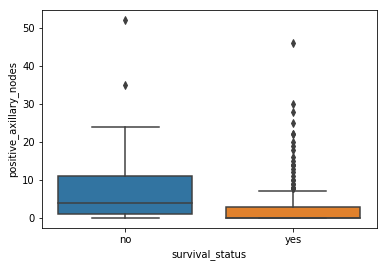
Observation(s)

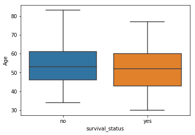
1. 75% of patients survived are of aged less than equal to 60.
2. 75% of patients survived have less than 4 axillary lymph nodes.
3. 75% of patients who have more have not survived have more than 10 axillary lymph nodes.

Data Preparation

Let’s divide the data set into two parts: train and test. Train data will be used to train the model and the performance of the model will be tested on the test data. For simplicity, we will use ‘Accuracy’ as the performance metric. In real-world scenarios, multiple technical metrics and business-specific KPIs are used to evaluate the model.

In [38]:
y=hman.survival_status
hman=hman.drop(columns=['survival_status'])
hman.head()

Out[38]:

	Age	year	positive_axillary_nodes
0	30	64	1
1	30	62	3
2	30	65	0
3	31	59	2
4	31	65	4

We will use 80% of data points for training purposes and 20% for testing. We will also use stratified sampling while doing the splits. It ensures the ratio of positive and negative classes will be the same in both train and test data.

In [53]:
# train,test: train and test data|y_train,y_test: train labels and test labels
train,test,y_train,y_test=train_test_split(hman,y,stratify=y,test_size=0.2)

Data Preprocessing

Real-world data sets are messy, it may contain thousands of missing values, null values, variables in a different scale, thousands of variables, etc. Data preprocessing is the set of methods to convert the raw data into a format on which data science algorithms can work. For this use case we will use a basic yet powerful data preprocessing technique called ‘Normalization’ which is nothing but converting the scales of the all variables in to a common scale (mean 0 standard deviation 1). We will use a very popular library called ‘ScikitLearn’ for this purpose.

In [54]:
# Normalizing the data using scikitLearn
nm=Normalizer()
train=nm.fit_transform(train)
test=nm.transform(test)

Model Training and Performance Evaluation

Here we will use a simple logistic regression model to predict the survival status. Logistic Regression is a very popular supervised machine learning algorithm that is used to solve classification problems.

In [61]:
# Model Training
clf=LogisticRegression(C=1.0,max_iter=500)
clf.fit(train,y_train)
Out[61]:
LogisticRegression(C=1.0, class_weight=None, dual=False, fit_intercept=True,
intercept_scaling=1, max_iter=500, multi_class='warn',
n_jobs=None, penalty='l2', random_state=None, solver='warn',
tol=0.0001, verbose=0, warm_start=False)
In [62]:
# Model Evaluation
y_pred=clf.predict(test)
accuracy_score(y_pred,y_test)

Out[62]:

0.7419354838709677

So using logistic regression on this data set we obtained an accuracy of 74%. In real-world scenarios we go through various stages of performance tuning over multiple algorithms and the best algorithm among those is chosen based on cross-validation score and other business requirements.

Conclusion

In this article, we have discussed the practical aspects of a data science use case at a very high level. In practice, the nature of use cases and data handling procedures will differ based on domain and business complexity.

Related Blogs

• Data Science Career Opportunities
• Data Science is Backbone of IT Industry?
• Data Science Career Opportunities